Retail case study
Walmart
Verifying In-store Footfall Accuracy Using Sales Performance Results
The correlation between model and the actual sales figures ρ=0.85, with a MAPE of 3.8%
This article shows how mobility data can be used to accurately predict net sales results for consumer- driven businesses like Walmart, the leading US big box retailer.
The Objective
The goal is to extract results from Huq Industries’ Footfall and Dwell-time modules that are highly correlated with the net sales figures published by Walmart in its quarterly trading updates. This output can then be incorporated into downstream models and systems to inform research for analysts and investors.
Step by Step Guide
Step 1: Get Walmart net sales data
Walmart publishes its net sales data within its quarterly trading updates, which can be found on its Investor Relations webpage. Note that for the purposes of this analysis, use is made only of the ‘Walmart US’ net sales segment.
Step 2: Find Walmart store visits
Huq’s mobility data serves as a proxy for consumer demand across Walmart’s US stores. This data is pre-enriched by Huq Industries in a process that extends raw geo-spatial data to include point of interest (POI) attributes such as business name, type and location.
Extracting Walmart visit data is therefore made easy by filtering on the raw place name (place_name), the standardised name (brand_name), or indeed by ignoring the POI attributes and using the WiFi SSID observed by the mobile device (impression_ssid) to match Walmart-specific patterns.
Step 3: Extract Walmart store visits
One way to quantify demand across the Walmart estate using Huq’s enriched geo-spatial data would be to count the number of distinct mobile devices (ie. panelists) present at Walmart each day. This approach can be useful in many analyses but after much experimentation there is a second strategy that produces results that more closely reflects behavioural nuance – and this is related to dwell.
During the same enrichment process that supplies the point-of-interest attributes, an estimate of dwell is also calculated and added to the resource. These properties can be accessed and manipulated via the columns impression_dwell_lower_bounds and impression_dwell_upper_bounds, which represent the upper and lower estimate for visit duration. These are calculated using the cumulative elapsed time calculated by continuous observations of a mobile device in the same place.
For the purposes of this study however, it is beneficial to develop a measurement of dwell that is less strict. The strategy used in this exercise groups observations into visits where they occur within 65 minutes of each other – without requiring them to be continuous per se.
Step 4: Test and training datasets
Walmart provides seventeen quarters of historical results via its investor portal. These are split into two sets; one to use for our training set and the other to test our output against. The training set helps us to select the optimal combination of parameters from the signal candidates described in Step 6. How this is evaluated is explored in Step 7.
The first twelve rows are chosen for training, and the remaining five are retained for testing. Separating them chronologically avoids test information leaking into the training process and causing lookahead bias.
Step 5: Define rough signal form
At this point take the training set from Step 4 then prepare it by eliminating behavioural outliers and concretely defining our measure of ‘dwell’.
i. Preparing the data
It is very common to find elements of noise within a dataset, and Huq’s enriched ‘Events’ feed is no exception. Some characteristics may be derived from interference at the sensor level; some artefacts may be behavioural and completely natural. As our demand metric relates to dwell, it is necessary to eliminate data points that show excessively little or large dwell before applying it. Filtering the data in this way excludes facets such as Walmart employees or other false positives derived from the enrichment process. Our chosen strategy filters the detected dwell value by an upper threshold Du , a lower threshold Dl and also determines whether to filter on a daily or per-visit basis, Db.
ii. Transform dwell into ‘demand signal’
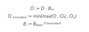
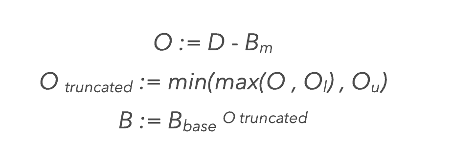
Let’s assume that dwell-time and spending money in- store is a non-linear relationship. Specifically, let’s suggest that there is a ‘normal’ level of dwell Bm and a ‘normal’ propensity for Walmart store visitors to spend, Bbase, both of which are constants.
We can then raise Bbase by the difference between the observed dwell value and the ‘normal’ value, Bm. To keep this value from exploding or vanishing, it is expedient to truncate the difference in the range of Ol to Ou before raising the power.
This can be summarised as follows:
iii. Normalise the data for panel growth
The size of Huq’s mobility panel changes over time as the number of apps supplying data increases, and apps’ own audience sizes fluctuate. As this study results in a time-series output, it is imperative to account for these changes in the normalised result so as to accurately represent the real trend. Similarly, it is also important to account for growth in the number of daily measurements observed per device using Huq’s measurement software in order to maintain a consistent view of ‘dwell’.
It may also help to consider how these characteristics vary geographically. The normalisation strategy employed in this exercise works by dividing the ‘demand signal’ observed across Walmart locations by the equivalent metric for the full US panel on equivalent day. This approach may be further improved by normalising on a localised basis to account for regional variations in data coverage, and by pre-filtering the data to remove individual app or panelist outliers.
iv. Respect seasonality in signal generation
Different week parts – weekdays, weekends and public holidays – have significance for in-store retail behaviour, and it is beneficial to recognise this in signal preparation. Accordingly, the normalised output is grouped using this classification, and is supplied to the model independently.
Step 6: Test and training datasets
The many possible combinations of parameters in Step 5 produce a huge number of candidates for signal representation, numbering 750K+. So, which candidate set offers the closest match to Walmart’s net sales values? A simple regression model (see Step 7) allows us to identify the best candidate set.
Step 7: Regression and validation
On the basis that we can expect longer dwell-times to lead to higher net sales results, a suitable model to use in this instance is non-negative least-squares regression as the inductive bias is well suited to this problem.
How do we know which signal output is best suited to net sales prediction? We’ll look for the result with the smallest mean absolute percentage error (MAPE), and use ‘leave-one-out cross validation’ to make best use of the limited supply of training data available in Walmart’s quarterly net sales figures archive.
The end result
The Pearson correlation between the output of the regression model and Walmart’s actual net sales figures on the (completely unseen) test set is ρ=0.85, with a MAPE of just 3.8%.
Conclusions
Using this parameter selection strategy it emerged that the optimal preparation steps and parameters are:
(i) remove dwell-time outliers, keeping daily device dwell values in the range of 0 to 160,
(ii) construct ‘demand signal’ by subtracting 30 from the daily dwell figure, and bound to the range of -12 to 60, then raise to the power of 1.03
(iii) normalise by counting 2hr-truncated timestamps across the full US dataset, where devices must have visited a non- residential location
Lastly, aggregate results by day and divide the ‘demand signal’ by this value.